ERC-4626: analyse performance of individual vaults
In this notebook, we examine a single or handful of handpicked ERC-4626 vaults
Vaults are picked manually by (chain, address) list
We analyse the vault performance by its share price, as reported by ERC-4626 smart contract interface.
We do last three months and historical all-time analyses
We look quantitative finance aspects of the vaults like returns, Sharpe and Sortino numbers
Some notes - Because of how vault metrics, share price and such are collected and interpreted, the results in this notebook contain various inaccuracies. - In this notebook, we use terms Net Asset Value (NAV) and Total Value Locked (TVL) interchangeably.
Usage
This is an open source notebook based on open data - You can edit and remix this notebook yourself
To do your own data research:
Read general instructions how to run the tutorials
See
ERC-4626: scanning vaults' historical price and performanceexample in tutorials first how to buildvault-prices-1h.parquetfile.
For any questions, follow and contact Trading Strategy community.
Setup
Set up notebook rendering output mode
Use static image charts so this notebook is readeable on Github / ReadTheDocs
[8]:
import pandas as pd
from plotly.offline import init_notebook_mode
import plotly.io as pio
from eth_defi.vault.base import VaultSpec
from eth_defi.research.notebook import set_large_plotly_chart_font
pd.options.display.float_format = "{:,.2f}".format
pd.options.display.max_columns = None
pd.options.display.max_rows = None
# Set up Plotly chart output as SVG
image_format = "png"
width = 1400
height = 800
# https://stackoverflow.com/a/52956402/315168
init_notebook_mode()
# https://plotly.com/python/renderers/#overriding-the-default-renderer
pio.renderers.default = image_format
current_renderer = pio.renderers[image_format]
# Have SVGs default pixel with
current_renderer.width = width
current_renderer.height = height
# Set all Plotly charts to use large font sizes for better readability,
# for sharing on mobile
set_large_plotly_chart_font(line_width=5, legend_font_size=16)
pio.templates.default = "custom"
Read and clean raw scanned vault price data
Read the Parquet file produced earlier with price scan
Clean the data if necessary
[9]:
from pathlib import Path
from eth_defi.vault.vaultdb import VaultDatabase
from eth_defi.vault.vaultdb import read_default_vault_prices
from eth_defi.vault.vaultdb import DEFAULT_RAW_PRICE_DATABASE
data_folder = Path("~/.tradingstrategy/vaults").expanduser()
vault_db = VaultDatabase.read()
prices_df = read_default_vault_prices()
print(prices_df.index.max())
print(f"Prices is {DEFAULT_RAW_PRICE_DATABASE}")
print(f"We have {len(vault_db):,} vaults in the database and {len(prices_df):,} price rows.")
2025-12-29 00:55:27
Prices is /Users/moo/.tradingstrategy/vaults/cleaned-vault-prices-1h.parquet
We have 26,576 vaults in the database and 5,953,190 price rows.
Choose vaults to examine
We pick vaults to examine and compare by chain and address tuples
[ ]:
from eth_defi.vault.base import VaultSpec
# Historically troublesome vaults
VAULTS = [
# atvPTmax
# VaultSpec(1, "0xd24e4a98b5fd90ff21a9cc5e2c1254de8084cd81"),
# TODO
VaultSpec(43114, "0x36e2aa296e798ca6262dc5fad5f5660e638d5402"),
# Valamor aUSD http://localhost:5173/trading-view/avalanche/vaults/varlamore-ausd-growth
VaultSpec(43114, "0x3d7b0c3997e48fa3fc96cd057d1fb4e5f891835b"),
# 1337
# VaultSpec(1, "0x94643e86aa5e38ddac6c7791c1297f4e40cd96c1"),
# yearn-v3-USDS-Farmer-USD
# VaultSpec(1, "0x39c0aec5738ed939876245224afc7e09c8480a52"),
# USDC Fluid Lender
# VaultSpec(1, "0x00c8a649c9837523ebb406ceb17a6378ab5c74cf"),
# Harvest USDC Autopilot on IPOR on Base
# https://app.ipor.io/fusion/base/0x0d877dc7c8fa3ad980dfdb18b48ec9f8768359c4/settings
# VaultSpec(8453, "0x0d877Dc7C8Fa3aD980DfDb18B48eC9F8768359C4"),
# IPOR USDC base
# https://app.ipor.io/fusion/base/0x45aa96f0b3188d47a1dafdbefce1db6b37f58216
# VaultSpec(8453, "0x45aa96f0b3188d47a1dafdbefce1db6b37f58216"),
# Summer.fi lazy
# VaultSpec(42161, "0x4f63cfea7458221cb3a0eee2f31f7424ad34bb58"),
# gTRADE (Gains) on Polygon
# https://app.ipor.io/fusion/base/0x45aa96f0b3188d47a1dafdbefce1db6b37f58216
# VaultSpec(137, "0x29019fe2e72e8d4d2118e8d0318bef389ffe2c81"),
# Gains on ARbitrum
# 42161-0xd85e038593d7a098614721eae955ec2022b9b91b
# VaultSpec(42161, "0xd85e038593d7a098614721eae955ec2022b9b91b"),
# gUSD on Arbitrum
# VaultSpec(42161, "0xd3443ee1e91af28e5fb858fbd0d72a63ba8046e0"),
# Peapods arbitrum
# VaultSpec(42161, "0xc2810eb57526df869049fbf4c541791a3255d24c"),
# Degen pool USDC 42161-0x20a1012b79e8f3ca3f802533c07934ef97398da
# VaultSpec(42161, "0x20a1012b79e8f3ca3f802533c07934ef97398da7"),
# Fluegel DAO
# 8453-0x277a3c57f3236a7d4548576074d7c3d7046eb26c
# https://fluegelcoin.com/dashboard
# VaultSpec(8453, "0x277a3c57f3236a7d4548576074d7c3d7046eb26c"),
# Plutus hedge on Arbitrum
# VaultSpec(42161, "0x58BfC95a864e18E8F3041D2FCD3418f48393fE6A"),
# crvUSD IBTC
# VaultSpec(42161, "0xe296ee7f83d1d95b3f7827ff1d08fe1e4cf09d8d"),
# D2 Hype on Arbitrum
# VaultSpec(42161, "0x75288264FDFEA8ce68e6D852696aB1cE2f3E5004"),
# Fluid on Ethereum
# VaultSpec(1, "0x00c8a649c9837523ebb406ceb17a6378ab5c74cf"),
# Upshift gamma
# VaultSpec(1, "0x998d7b14c123c1982404562b68eddb057b0477cb"),
]
Period selection
Choose the period we want to examine
Comment out the trim operation if you want to examine the latest data
[11]:
last_sample_at = prices_df.index.max()
three_months_ago = last_sample_at - pd.DateOffset(months=3)
PERIOD = [
three_months_ago,
last_sample_at,
]
print(f"Trimming price data to period from {PERIOD[0]} to {PERIOD[1]}.")
mask = (prices_df.index >= PERIOD[0]) & (prices_df.index <= PERIOD[1])
prices_df = prices_df[mask]
print(f"Trimmed period contains {len(prices_df):,} price rows.")
prices_df = prices_df.sort_index()
display(prices_df.tail(2))
Trimming price data to period from 2025-09-29 00:55:27 to 2025-12-29 00:55:27.
Trimmed period contains 969,491 price rows.
| id | chain | address | block_number | share_price | total_assets | total_supply | performance_fee | management_fee | errors | name | event_count | protocol | raw_share_price | returns_1h | avg_assets_by_vault | dynamic_tvl_threshold | tvl_filtering_mask | |
|---|---|---|---|---|---|---|---|---|---|---|---|---|---|---|---|---|---|---|
| timestamp | ||||||||||||||||||
| 2025-12-29 00:55:27 | 10-0x6926b434cce9b5b7966ae1bfeef6d0a7dcf3a8bb | 10 | 0x6926b434cce9b5b7966ae1bfeef6d0a7dcf3a8bb | 145685475 | 1.09 | 1,882,561.42 | 1,727,893.56 | NaN | NaN | exactly USDC | 226488 | <protocol not yet identified> | 1.09 | 0.00 | 4,566,831.10 | 91,336.62 | False | |
| 2025-12-29 00:55:27 | 10-0x035c93db04e5aaea54e6cd0261c492a3e0638b37 | 10 | 0x035c93db04e5aaea54e6cd0261c492a3e0638b37 | 145685475 | 1.21 | 49,705.69 | 40,986.76 | NaN | NaN | Static Aave Optimism USDT | 33407 | Superform | 1.21 | 0.00 | 40,618.50 | 812.37 | False |
Examine data
Examine metadata
[12]:
examined_vault_spec = VAULTS[0]
examined_id = f"{examined_vault_spec.chain_id}-{examined_vault_spec.vault_address}"
vault_metadata = vault_db.rows[examined_vault_spec]
display(vault_metadata)
{'Symbol': 'TIDAVAY_USDC',
'Name': 'TiD Capital Avalanche Yield',
'Address': '0x36e2aa296e798ca6262dc5fad5f5660e638d5402',
'Denomination': 'USDC',
'Share token': 'TIDAVAY_USDC',
'NAV': Decimal('67801.754191'),
'Protocol': '<protocol not yet identified>',
'Mgmt fee': None,
'Perf fee': None,
'Deposit fee': None,
'Withdraw fee': None,
'Shares': Decimal('14232270910.974665'),
'First seen': datetime.datetime(2025, 9, 27, 7, 51, 43),
'Features': '',
'Link': 'https://routescan.io/address/0x36E2AA296E798Ca6262DC5Fad5F5660e638d5402',
'_detection_data': ERC4262VaultDetection(chain=43114, address='0x36e2aa296e798ca6262dc5fad5f5660e638d5402', first_seen_at_block=69371655, first_seen_at=datetime.datetime(2025, 9, 27, 7, 51, 43), features=set(), updated_at=datetime.datetime(2025, 12, 29, 0, 50, 4, 453740), deposit_count=15, redeem_count=13),
'_denomination_token': {'name': 'USD Coin',
'symbol': 'USDC',
'total_supply': 569693925223775,
'decimals': 6,
'extra_data': {'cached': True},
'address': '0xB97EF9Ef8734C71904D8002F8b6Bc66Dd9c48a6E',
'chain': 43114},
'_share_token': {'name': 'TiD Capital Avalanche Yield',
'symbol': 'TIDAVAY_USDC',
'total_supply': 14232270910974665,
'decimals': 6,
'extra_data': {'cached': True},
'address': '0x36E2AA296E798Ca6262DC5Fad5F5660e638d5402',
'chain': 43114},
'_fees': FeeData(fee_mode=None, management=None, performance=None, deposit=None, withdraw=None),
'_flags': set(),
'_lockup': None}
Vault charts and performance tearsheets
Examine vault metrics and charts
[14]:
from eth_defi.research.vault_metrics import analyse_vault, format_ffn_performance_stats
from eth_defi.chain import get_chain_name
from IPython.display import display, HTML
for vault_spec in VAULTS:
vault_report = analyse_vault(
vault_db=vault_db,
prices_df=prices_df,
spec=vault_spec,
chart_frequency="daily",
)
chain_name = get_chain_name(vault_spec.chain_id)
vault_name = vault_report.vault_metadata["Name"]
print(f"Analysing vault {vault_name} ({chain_name}): {vault_spec.as_string_id()}")
display(HTML(f"<h2>Vault {vault_name} ({chain_name}): {vault_spec.vault_address})</h2><br>"))
# Display returns figur
returns_chart_fig = vault_report.rolling_returns_chart
returns_chart_fig.show()
# Check raw montly share price numbers for each vault
hourly_price_df = vault_report.hourly_df
last_price_at = hourly_price_df.index[-1]
last_price = hourly_price_df["share_price"].asof(last_price_at)
last_block = hourly_price_df["block_number"].asof(last_price_at)
month_ago = last_price_at - pd.DateOffset(months=1)
month_ago_price = hourly_price_df["share_price"].asof(month_ago)
month_ago_block = hourly_price_df["block_number"].asof(month_ago)
if not pd.isna(month_ago_price):
print(f"Vault {vault_spec.chain_id}-{vault_spec.vault_address}: no price data for month ago {month_ago} found, last price at {last_price_at} is {last_price}")
continue
data = {
"Vault": f"{vault_name} ({chain_name})",
"Last price at": last_price_at,
"Last price": last_price,
"Block last price": f"{month_ago_block:,}",
"Month ago": month_ago,
"Block month ago": f"{month_ago_block:,}",
"Month ago price": month_ago_price,
"Monthly change %": (last_price - month_ago_price) / month_ago_price * 100,
}
df = pd.Series(data)
display(df)
# Display FFN stats
performance_stats = vault_report.performance_stats
if performance_stats is not None:
stats_df = format_ffn_performance_stats(performance_stats)
# display(stats_df)
display(HTML(stats_df.to_frame(name='Value').to_html(float_format='{:,.2f}'.format, index=True)))
else:
print(f"Vault {vault_spec.chain_id}-{vault_spec.vault_address}: performance metrics not available, is quantstats library installed?")
Share price movement: 0.0000 2025-09-29 15:00:00 -> 0.0000 2025-12-28 23:00:00
Analysing vault TiD Capital Avalanche Yield (Avalanche): 43114-0x36e2aa296e798ca6262dc5fad5f5660e638d5402
Vault TiD Capital Avalanche Yield (Avalanche): 0x36e2aa296e798ca6262dc5fad5f5660e638d5402)
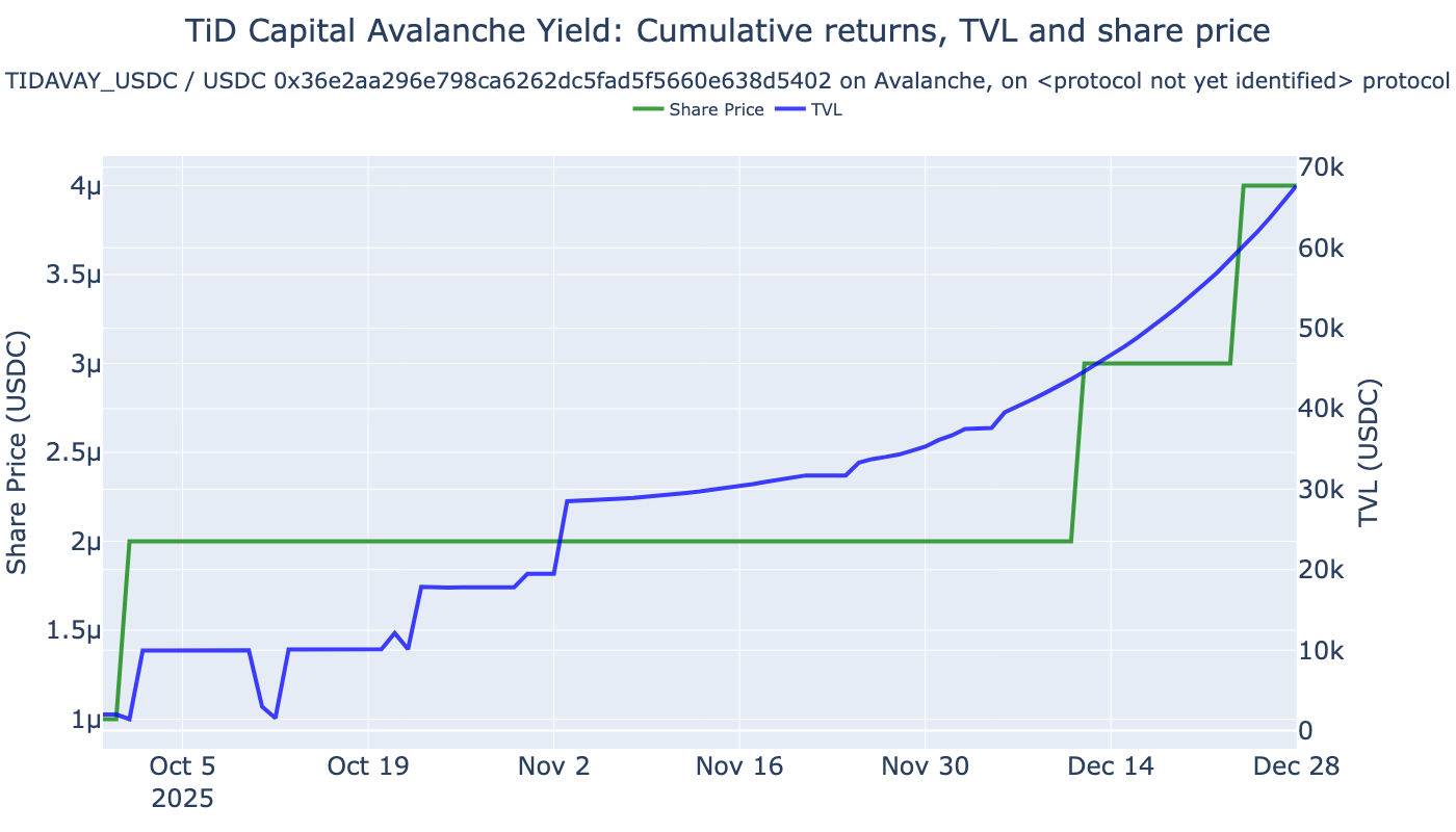
Vault 43114-0x36e2aa296e798ca6262dc5fad5f5660e638d5402: no price data for month ago 2025-11-28 23:00:00 found, last price at 2025-12-28 23:00:00 is 4e-06
---------------------------------------------------------------------------
AssertionError Traceback (most recent call last)
Cell In[14], line 8
4 from IPython.display import display, HTML
6 for vault_spec in VAULTS:
----> 8 vault_report = analyse_vault(
9 vault_db=vault_db,
10 prices_df=prices_df,
11 spec=vault_spec,
12 chart_frequency="daily",
13 )
15 chain_name = get_chain_name(vault_spec.chain_id)
16 vault_name = vault_report.vault_metadata["Name"]
File ~/code/trade-executor/deps/web3-ethereum-defi/eth_defi/research/vault_metrics.py:1268, in analyse_vault(vault_db, prices_df, spec, returns_col, logger, chart_frequency)
1266 vault_metadata = vault_db.get(spec)
1267 if vault_metadata is None:
-> 1268 assert vault_metadata, f"Vault with id {spec} not found in vault database"
1270 chain_name = get_chain_name(spec.chain_id)
1271 name = vault_metadata["Name"]
AssertionError: Vault with id VaultSpec(chain_id=43114, vault_address='0x3d7b0c3997e48fa3fc96cd057d1fb4e5f891835b1') not found in vault database
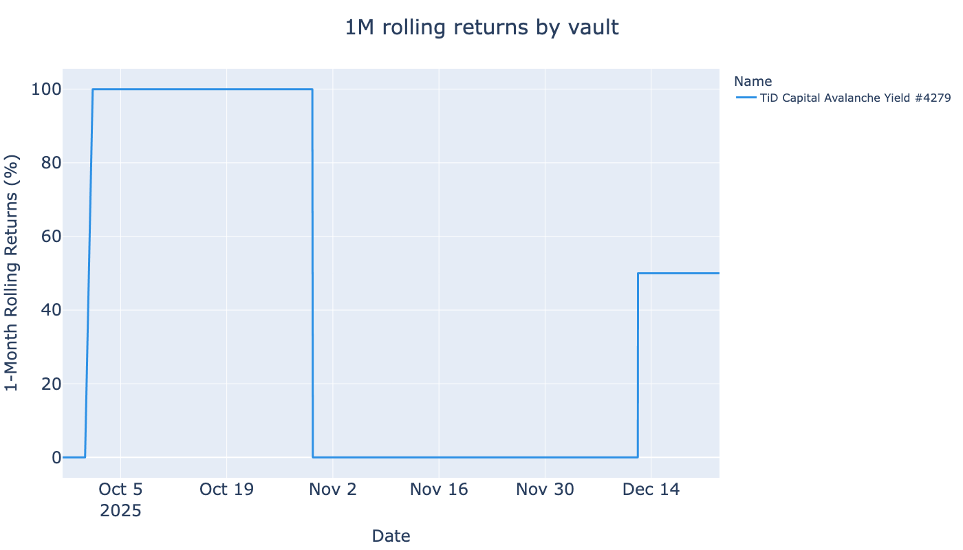
Rolling returns comparison
Show rolling returns of all picked vaults
[ ]:
from eth_defi.research.rolling_returns import calculate_rolling_returns, visualise_rolling_returns
interesting_vaults = [spec.as_string_id() for spec in VAULTS]
rolling_returns_df = calculate_rolling_returns(
prices_df,
interesting_vaults=interesting_vaults,
clip_up=100,
)
display(rolling_returns_df.head(3))
fig = visualise_rolling_returns(rolling_returns_df)
fig.show()
| id | timestamp | chain | address | block_number | share_price | total_assets | total_supply | performance_fee | management_fee | errors | name | event_count | protocol | raw_share_price | returns_1h | avg_assets_by_vault | dynamic_tvl_threshold | tvl_filtering_mask | rolling_1m_returns | |
|---|---|---|---|---|---|---|---|---|---|---|---|---|---|---|---|---|---|---|---|---|
| 0 | 43114-0x36e2aa296e798ca6262dc5fad5f5660e638d5402 | 2025-09-27 08:10:55 | 43114 | 0x36e2aa296e798ca6262dc5fad5f5660e638d5402 | 69372297 | 0.00 | 2,000.00 | 2,000,000,000.00 | NaN | NaN | TiD Capital Avalanche Yield #4279 | 28 | <protocol not yet identified> | 0.00 | NaN | 23,645.82 | 472.92 | False | 0.00 | |
| 1 | 43114-0x36e2aa296e798ca6262dc5fad5f5660e638d5402 | 2025-09-27 09:02:48 | 43114 | 0x36e2aa296e798ca6262dc5fad5f5660e638d5402 | 69374097 | 0.00 | 2,000.02 | 2,000,000,000.00 | NaN | NaN | TiD Capital Avalanche Yield #4279 | 28 | <protocol not yet identified> | 0.00 | 0.00 | 23,645.82 | 472.92 | False | 0.00 | |
| 2 | 43114-0x36e2aa296e798ca6262dc5fad5f5660e638d5402 | 2025-09-27 09:51:12 | 43114 | 0x36e2aa296e798ca6262dc5fad5f5660e638d5402 | 69375897 | 0.00 | 2,000.02 | 2,000,000,000.00 | NaN | NaN | TiD Capital Avalanche Yield #4279 | 28 | <protocol not yet identified> | 0.00 | 0.00 | 23,645.82 | 472.92 | False | 0.00 |
Raw vault data
Examine raw data of a single vault
Find abnormal return rows
[ ]:
# Fluegel DAO
# 8453-0x277a3c57f3236a7d4548576074d7c3d7046eb26c
# https://fluegelcoin.com/dashboard
vault_spec = VaultSpec(8453, "0x277a3c57f3236a7d4548576074d7c3d7046eb26c")
df = prices_df[prices_df["id"] == vault_spec.as_string_id()]
# 10% claimed hourly returns
mask = df["returns_1h"].abs() > 0.10
expanded_mask = (mask | mask.shift(1) | mask.shift(-1)).fillna(False)
df = df[expanded_mask] # Filter out rows with small returns
display(df.head(10))
| id | chain | address | block_number | share_price | total_assets | total_supply | performance_fee | management_fee | errors | name | event_count | protocol | raw_share_price | returns_1h | avg_assets_by_vault | dynamic_tvl_threshold | tvl_filtering_mask | |
|---|---|---|---|---|---|---|---|---|---|---|---|---|---|---|---|---|---|---|
| timestamp | ||||||||||||||||||
| 2025-09-24 08:36:07 | 8453-0x277a3c57f3236a7d4548576074d7c3d7046eb26c | 8453 | 0x277a3c57f3236a7d4548576074d7c3d7046eb26c | 35956810 | 2.04 | 661,538.44 | 323,616.44 | NaN | NaN | Fluegel DAO (Base) #248 | 555 | <protocol not yet identified> | 2.04 | -0.00 | 603,195.56 | 12,063.91 | False | |
| 2025-09-24 10:36:07 | 8453-0x277a3c57f3236a7d4548576074d7c3d7046eb26c | 8453 | 0x277a3c57f3236a7d4548576074d7c3d7046eb26c | 35960410 | 1.82 | 588,709.80 | 323,616.44 | NaN | NaN | Fluegel DAO (Base) #248 | 555 | <protocol not yet identified> | 1.82 | -0.11 | 603,195.56 | 12,063.91 | False | |
| 2025-09-24 11:36:07 | 8453-0x277a3c57f3236a7d4548576074d7c3d7046eb26c | 8453 | 0x277a3c57f3236a7d4548576074d7c3d7046eb26c | 35962210 | 2.07 | 669,008.32 | 323,616.44 | NaN | NaN | Fluegel DAO (Base) #248 | 555 | <protocol not yet identified> | 2.07 | 0.14 | 603,195.56 | 12,063.91 | False | |
| 2025-09-24 13:36:07 | 8453-0x277a3c57f3236a7d4548576074d7c3d7046eb26c | 8453 | 0x277a3c57f3236a7d4548576074d7c3d7046eb26c | 35965810 | 2.06 | 667,852.18 | 323,616.44 | NaN | NaN | Fluegel DAO (Base) #248 | 555 | <protocol not yet identified> | 2.06 | -0.00 | 603,195.56 | 12,063.91 | False | |
| 2025-10-01 17:36:07 | 8453-0x277a3c57f3236a7d4548576074d7c3d7046eb26c | 8453 | 0x277a3c57f3236a7d4548576074d7c3d7046eb26c | 36275410 | 2.25 | 727,138.15 | 323,616.44 | NaN | NaN | Fluegel DAO (Base) #248 | 555 | <protocol not yet identified> | 2.25 | -0.01 | 603,195.56 | 12,063.91 | False | |
| 2025-10-01 18:36:07 | 8453-0x277a3c57f3236a7d4548576074d7c3d7046eb26c | 8453 | 0x277a3c57f3236a7d4548576074d7c3d7046eb26c | 36277210 | 1.99 | 644,306.79 | 323,616.44 | NaN | NaN | Fluegel DAO (Base) #248 | 555 | <protocol not yet identified> | 1.99 | -0.11 | 603,195.56 | 12,063.91 | False | |
| 2025-10-01 19:36:07 | 8453-0x277a3c57f3236a7d4548576074d7c3d7046eb26c | 8453 | 0x277a3c57f3236a7d4548576074d7c3d7046eb26c | 36279010 | 2.25 | 728,047.48 | 323,616.44 | NaN | NaN | Fluegel DAO (Base) #248 | 555 | <protocol not yet identified> | 2.25 | 0.13 | 603,195.56 | 12,063.91 | False | |
| 2025-10-01 20:36:07 | 8453-0x277a3c57f3236a7d4548576074d7c3d7046eb26c | 8453 | 0x277a3c57f3236a7d4548576074d7c3d7046eb26c | 36280810 | 2.24 | 725,813.95 | 323,616.44 | NaN | NaN | Fluegel DAO (Base) #248 | 555 | <protocol not yet identified> | 2.24 | -0.00 | 603,195.56 | 12,063.91 | False | |
| 2025-10-01 22:36:07 | 8453-0x277a3c57f3236a7d4548576074d7c3d7046eb26c | 8453 | 0x277a3c57f3236a7d4548576074d7c3d7046eb26c | 36284410 | 2.27 | 733,985.44 | 323,616.44 | NaN | NaN | Fluegel DAO (Base) #248 | 555 | <protocol not yet identified> | 2.27 | 0.00 | 603,195.56 | 12,063.91 | False | |
| 2025-10-01 23:36:07 | 8453-0x277a3c57f3236a7d4548576074d7c3d7046eb26c | 8453 | 0x277a3c57f3236a7d4548576074d7c3d7046eb26c | 36286210 | 2.03 | 655,645.90 | 323,616.44 | NaN | NaN | Fluegel DAO (Base) #248 | 555 | <protocol not yet identified> | 2.03 | -0.11 | 603,195.56 | 12,063.91 | False |