Derive historical open interest and funding rate

Derive is a decentralised options and perpetual futures exchange built on its own OP Stack L2 chain (Derive Chain, chain ID 957). This notebook visualises historical open interest and funding rate data for BTC and ETH perpetual contracts.

• Open interest measures the total outstanding perpetual positions (in base currency units, e.g. BTC or ETH). It is read from on-chain state via Multicall3.

• Funding rate is the hourly rate paid between longs and shorts to keep the perpetual price anchored to the index price. It is fetched from Derive’s REST API.

For full details on the Derive integration, data sources, API quirks and scan scripts, see README-derive.md.

Populating the DuckDB database

This notebook reads from a local DuckDB database at ~/.tradingstrategy/derive/funding-rates.duckdb. You must populate it before running the notebook by executing the two scan scripts:

1. Scan funding rates (hourly snapshots from Derive REST API, ~2-3 min for full history):

poetry run python scripts/derive/scan-funding-rates.py

2. Scan open interest (daily on-chain snapshots via Multicall3, ~20 min for full backfill):

poetry run python scripts/derive/scan-open-interest.py

Both scripts are incremental — subsequent runs only fetch new data since the last sync. You can limit the sync to specific instruments with INSTRUMENTS=ETH-PERP,BTC-PERP or control the database path with DB_PATH. See README-derive.md for all environment variables and performance benchmarks.

Running this notebook

Run from the command line:

poetry run jupyter execute docs/source/tutorials/derive-open-interest-funding-rate.ipynb --inplace --timeout=900

Or open in Visual Studio Code / JupyterLab.

# Set up static PNG chart output
from eth_defi.research.notebook import setup_charting_and_output, OutputMode, set_large_plotly_chart_font

setup_charting_and_output(OutputMode.static, image_format="png", width=1500, height=800, increase_font_size=False)
set_large_plotly_chart_font()

import datetime

import pandas as pd
import plotly.graph_objects as go
from plotly.subplots import make_subplots

from eth_defi.derive.historical import DeriveFundingRateDatabase

Load data from local DuckDB

db = DeriveFundingRateDatabase()
start_time = datetime.datetime(2025, 1, 1)

# Fetch open interest DataFrames (columns: timestamp, instrument, open_interest, perp_price, index_price)
btc_oi_df = db.get_open_interest_dataframe("BTC-PERP", start_time=start_time)
eth_oi_df = db.get_open_interest_dataframe("ETH-PERP", start_time=start_time)

# Fetch funding rate DataFrames (columns: timestamp, instrument, funding_rate)
btc_fr_df = db.get_funding_rates_dataframe("BTC-PERP", start_time=start_time)
eth_fr_df = db.get_funding_rates_dataframe("ETH-PERP", start_time=start_time)

db.close()

# Compute OI in USD terms using index price
btc_oi_df["oi_usd"] = btc_oi_df["open_interest"].astype(float) * btc_oi_df["index_price"].astype(float)
eth_oi_df["oi_usd"] = eth_oi_df["open_interest"].astype(float) * eth_oi_df["index_price"].astype(float)

# Resample hourly funding rates to daily mean for cleaner charts
btc_fr_daily = btc_fr_df.set_index("timestamp")["funding_rate"].resample("1D").mean().reset_index()
eth_fr_daily = eth_fr_df.set_index("timestamp")["funding_rate"].resample("1D").mean().reset_index()

summary = pd.DataFrame({
    "Instrument": ["BTC-PERP", "ETH-PERP"],
    "OI rows": [len(btc_oi_df), len(eth_oi_df)],
    "Funding rate rows": [len(btc_fr_df), len(eth_fr_df)],
    "OI date range": [
        f"{btc_oi_df['timestamp'].min()} - {btc_oi_df['timestamp'].max()}",
        f"{eth_oi_df['timestamp'].min()} - {eth_oi_df['timestamp'].max()}",
    ],
})
display(summary)

	Instrument	OI rows	Funding rate rows	OI date range
0	BTC-PERP	10630	10636	2025-01-01 00:00:01 - 2026-03-19 21:00:01
1	ETH-PERP	10630	10637	2025-01-01 00:00:01 - 2026-03-19 21:00:01

Summary metrics

def compute_metrics(fr_df: pd.DataFrame, oi_df: pd.DataFrame, name: str) -> dict:
    """Compute funding rate and OI metrics for one instrument."""
    fr = fr_df["funding_rate"].astype(float)
    hours_positive = int((fr > 0).sum())
    hours_negative = int((fr < 0).sum())
    total_hours = len(fr)
    mean_hourly = fr.mean()

    oi_usd = oi_df["oi_usd"]
    return {
        "Instrument": name,
        "Hours positive": f"{hours_positive:,}",
        "Hours negative": f"{hours_negative:,}",
        "% hours positive": f"{100 * hours_positive / total_hours:.1f}%",
        "Mean hourly rate": f"{mean_hourly:.8f}",
        "Annualised rate": f"{mean_hourly * 8760:.2%}",
        "Max hourly rate": f"{fr.max():.8f}",
        "Min hourly rate": f"{fr.min():.8f}",
        "Cumulative funding": f"{fr.sum():.4f}",
        "Current OI (USD)": f"${oi_usd.iloc[-1]:,.0f}",
        "Peak OI (USD)": f"${oi_usd.max():,.0f}",
        "Mean OI (USD)": f"${oi_usd.mean():,.0f}",
    }

metrics = pd.DataFrame([
    compute_metrics(btc_fr_df, btc_oi_df, "BTC-PERP"),
    compute_metrics(eth_fr_df, eth_oi_df, "ETH-PERP"),
]).set_index("Instrument").T
metrics.index.name = None
display(metrics)

Instrument	BTC-PERP	ETH-PERP
Hours positive	8,718	8,987
Hours negative	1,918	1,650
% hours positive	82.0%	84.5%
Mean hourly rate	0.00001250	0.00001131
Annualised rate	10.95%	9.91%
Max hourly rate	0.00045662	0.00078069
Min hourly rate	-0.00021506	-0.00034533
Cumulative funding	0.1330	0.1203
Current OI (USD)	$25,622,330	$7,181,877
Peak OI (USD)	$26,845,258	$22,495,469
Mean OI (USD)	$11,685,941	$8,303,178

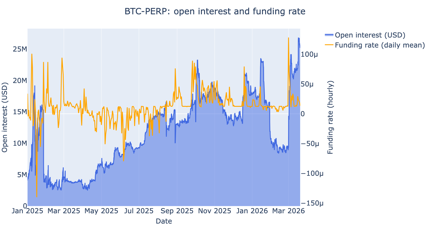
BTC open interest and funding rate

fig = make_subplots(specs=[[{"secondary_y": True}]])

# Open interest in USD on left y-axis
fig.add_trace(
    go.Scatter(
        x=btc_oi_df["timestamp"],
        y=btc_oi_df["oi_usd"],
        name="Open interest (USD)",
        fill="tozeroy",
        line=dict(color="royalblue"),
    ),
    secondary_y=False,
)

# Daily mean funding rate on right y-axis
fig.add_trace(
    go.Scatter(
        x=btc_fr_daily["timestamp"],
        y=btc_fr_daily["funding_rate"].astype(float),
        name="Funding rate (daily mean)",
        line=dict(color="orange"),
    ),
    secondary_y=True,
)

fig.update_layout(title="BTC-PERP: open interest and funding rate", height=600)
fig.update_yaxes(title_text="Open interest (USD)", secondary_y=False, showgrid=False)
fig.update_yaxes(title_text="Funding rate (hourly)", secondary_y=True, showgrid=False)
fig.update_xaxes(title_text="Date")
fig.show()

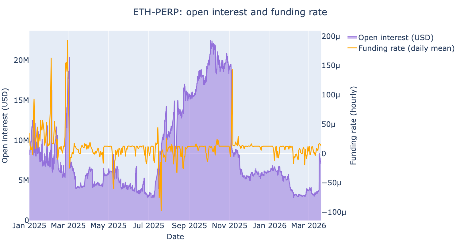
ETH open interest and funding rate

fig = make_subplots(specs=[[{"secondary_y": True}]])

# Open interest in USD on left y-axis
fig.add_trace(
    go.Scatter(
        x=eth_oi_df["timestamp"],
        y=eth_oi_df["oi_usd"],
        name="Open interest (USD)",
        fill="tozeroy",
        line=dict(color="mediumpurple"),
    ),
    secondary_y=False,
)

# Daily mean funding rate on right y-axis
fig.add_trace(
    go.Scatter(
        x=eth_fr_daily["timestamp"],
        y=eth_fr_daily["funding_rate"].astype(float),
        name="Funding rate (daily mean)",
        line=dict(color="orange"),
    ),
    secondary_y=True,
)

fig.update_layout(title="ETH-PERP: open interest and funding rate", height=600)
fig.update_yaxes(title_text="Open interest (USD)", secondary_y=False, showgrid=False)
fig.update_yaxes(title_text="Funding rate (hourly)", secondary_y=True, showgrid=False)
fig.update_xaxes(title_text="Date")
fig.show()